Hey all! Today's post is provided by guest contributor Jerry Shelton. Jerry is a Project Manager at Hewlett Packard as well as an HP Sigma Plus Certified Black Belt. Lucky for us, he has provided a wonderful example of how to take a date/time stamp from a data set that was exported from a database and determine the beginning of the week to allow for simple grouping within a pivot table/chart.
This solution is a real-world example that was born out of the need of others that were not too excel savvy to create reports from data sources with similar formatting. This template allows them to simply copy/paste the formulas shown in this example into their own data and move from there with very little training or guidance from others. I fully support making life easier for others!
Here's a link to the file with the "How To" included inside:
Beginning of Week - Formula Example
**Note: The above file does not contain Macros.
Cheers!
Tuesday, March 25, 2014
Friday, March 21, 2014
Concatenation and Searching for text in a string
Today I was asked to create a unique identifier by obtaining the initials of a name and adding on the last 4 digits of a specific encounter number. This required the following functions:
Left(text, [num chars])
Mid(text, start_num, num_chars)
Right(text, [num_chars])
Search(find_text, within_text, [start_num])
and the symbol used to concatenate values/strings: "&"
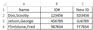
Here's the dataset:

Here we have the names list by LastName,FirstName and the ID#'s.
The assignment: "Provide Initials (First then Last) and the last 4 digits in the ID#"
**For this example, we're going to assume all of the names are in the exact same format down every row.
Let's Begin:
In Cell C1 we'll provide a column header of "New ID". In cell C2 we'll go to the formula bar and begin with our formula. Since the First initial is in the MIDDLE of the text string and and be found after a comma, we'll use the Mid() and Search() formulas here.
For the MID() formula we need to assign values to the following requirements -
=MID(A2,SEARCH(",",A2,1)+1,1)
This returns "S" in cell C2. Next, we need the First letter of the Last Name. This one is a bit more simple since it is the beginning letter of the text string. We'll use the LEFT() formula
For the LEFT() formula, we need to assign values to the following requirements:

The task I had to accomplish was a bit more complicated involving dates of service as well. The last step that you would want to do is validate that the "New ID" was truly unique across your data set. To accomplish this, you could simply create a pivot table, add the "New ID" and then Name as the Row values and add New ID to the values section as a count of New ID. This would quickly show if you have any duplicates by listing multiple names under the same ID.
Hope you enjoyed this tutorial! Instead of offering to donate lots of your money to me, let other people do it by clicking on an advertisement to the right!
Left(text, [num chars])
Mid(text, start_num, num_chars)
Right(text, [num_chars])
Search(find_text, within_text, [start_num])
and the symbol used to concatenate values/strings: "&"
Here's the dataset:
Here we have the names list by LastName,FirstName and the ID#'s.
The assignment: "Provide Initials (First then Last) and the last 4 digits in the ID#"
**For this example, we're going to assume all of the names are in the exact same format down every row.
Let's Begin:
In Cell C1 we'll provide a column header of "New ID". In cell C2 we'll go to the formula bar and begin with our formula. Since the First initial is in the MIDDLE of the text string and and be found after a comma, we'll use the Mid() and Search() formulas here.
For the MID() formula we need to assign values to the following requirements -
- text: the text we're referencing is the Name column and found in cell A2
- start_num: we need to search for the "," and start with the character immediately after it (+1)
- Search requires the following to be addressed:
- Find_text or Text to search for: "," (include the "" around the comma in the formula for this one)
- within_text: cell A2
- [start_num]: "1" - this is the first character in the cell A2
- num_chars: 1 - we only want the first letter of the first name
So, now that we have this written out in words, let's convert it to the formula:
=MID(A2,SEARCH(",",A2,1)+1,1)
This returns "S" in cell C2. Next, we need the First letter of the Last Name. This one is a bit more simple since it is the beginning letter of the text string. We'll use the LEFT() formula
For the LEFT() formula, we need to assign values to the following requirements:
- Text: A2
- [num_chars]: 1
This will provide the first character from the left using the value in cell A2. The formula looks like this:
=LEFT(A2,1)
So, we want all of this in one cell, right? How do we enter more than one formula? Concatenation!
All we have to do is combine the two formulas by replacing the "=" at the beginning of the second formula with "&" and append it to the end of the first formula:
=MID(A2,SEARCH(",",A2,1)+1,1)&LEFT(A2,1)
This now returns "SD" in cell C2. Last, we need the last four numbers in the ID#: We'll use the RIGHT() formula to accomplish this task:
For the RIGHT() formula, we need to assign values to the following requirements:
**Instead of looking at the left of the text, this formula starts at the right**
- Text: B2 - not A2, because the numbers are in B2!
- [num_chars]: 4
This will provide the first four characters from the right using the value in cell B2. The formula looks like this:
=RIGHT(B2,4)
Again, we want all of this in one cell, right? Let's concatenate by replacing the "=" with "&" and appending it to the end of the formula we've built so far:
=MID(A2,SEARCH(",",A2,1)+1,1)&LEFT(A2,1)&RIGHT(B2,4)
This now returns "SD3456" in cell C2. Let's look back at the assignment: "Provide Initials (First then Last) and the last 4 digits in the ID#"
Now that we know we've accomplished what we wanted, we can copy the values down the column and click SAVE!
The final result:
AND the final result showing the formulas used:
The task I had to accomplish was a bit more complicated involving dates of service as well. The last step that you would want to do is validate that the "New ID" was truly unique across your data set. To accomplish this, you could simply create a pivot table, add the "New ID" and then Name as the Row values and add New ID to the values section as a count of New ID. This would quickly show if you have any duplicates by listing multiple names under the same ID.
Hope you enjoyed this tutorial! Instead of offering to donate lots of your money to me, let other people do it by clicking on an advertisement to the right!
Tuesday, March 18, 2014
PowerPivot: BLANK() & ISBLANK()
Today I ran into an issue when writing a formula in the calculated column area. I needed to calculate the difference in minutes between two date/time columns. However, I first wanted to check to be sure both columns in the row had an entry to avoid some outrageous number appearing as the result of the formula.
In excel I would have simply handled this issue with an If() Statement check to be sure the cell wasn't blank and then returning "" if it was.
The formula in an Excel spreadsheet looks like this:
=if(A1="","",if(A2="","",(A2-A1)*24*60))
Unfortunately, when used in the data model this will return "#Error" for all rows in the column instead of a blank value.
After consulting with a coworker, he showed me how he has resolved this issue:
=If(ISBLANK([Column1]),BLANK(),if(ISBLANK([Column2]),BLANK(),([Column2]-[Column1])*24*60))
The ISBLANK() formula simply checks to see if the value in the column is blank. If it is, BLANK() returns the value as a blank cell - Much the same as using "" in an Excel Sheet formula.
To Explain the formula, I will write it in words:
If the value on this row of column1 is blank then return blank, otherwise go check if the value on this row of column2 is blank. If it is, return blank, otherwise calculate the difference between Date2 and Date1. Multiply the result by 24 to get hours. Multply the hours by 60 to get minutes.
Hope this helps someone else save some time!
Thursday, March 6, 2014
Question for the Audience...
Okay all, I have a problem that I don't know how to fix. HUGE points to one who has an appropriate solution.
The Problem: How do I default a text value slicer selection WITHOUT using VBA? Is it even possible?
Why no VBA? Our company is a bit behind the times in upgrading us all to the same version of office. I have Excel 2013, but the rest of the world is using 2007 (No slicers available). Therefore, I post my files to a SharePoint site and the end users are able to use them via Excel Services (hence the no VBA).
I am searching all over for this answer right now and will gladly share the how-to if/when I figure it out. I would gladly host a "Guest Post" if you know how to do this already.
Thanks!
Subscribe to:
Posts (Atom)