The other day I was called into an issue where the user needed a formula that would look up the results of specific tests based on the month that they were run. He wanted to enter a month into a cell and the formulas would return the values of the tests for that month. In response, I created a demo spreadsheet (No Macros) to show him how to get the result he wanted.
His initial question was "Is there a way to do this VLOOKUP()?". Yes, this could be accomplished with VLOOKUP() assuming the tables were organized appropriately, but I wanted to introduce a new method. VLOOKUP()is a great formula, but has it's limitations. For example, Column1 of the table referenced when looking for a specific value MUST be the left-most array column that contains that value...
While I'm sure there would be a convoluted way to go about accomplishing that task by counting the month from an original start date and using that as the column reference in the VLOOKUP() formula, I felt it would be a better time to use the INDEX() and MATCH() formulas to find the intersections of row and column.
Here's how I accomplished it:
Formulas:
INDEX(array, row_num, [column_num])
MATCH(lookup_value, lookup_array, [match type])
Data Set:
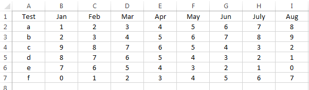
The user's file was set up so the column contains the test name (run only once per month and not duplicated) and the following columns are the results of the tests under each month.
Now, off to the right of the data set, I created an example of how to set up a quick reference for the month's data:
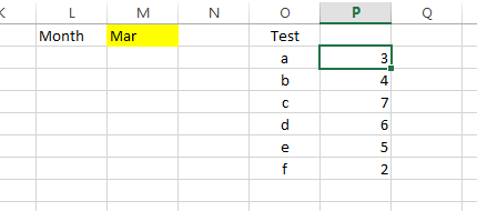
The Yellow cell is where the month is entered and cells P2:P7 contain the formulas that refer to the month and test name to return the appropriate value.
On to the formula... In cell P2, Start with the INDEX() formula. The array is the data table in cells A1:I7 so we now have:
=INDEX($A$2:$I$7,
The next step is to identify which row we're interested in. We use the MATCH() formula for this. The items we need for MATCH() are:
Lookup_value = O2 (this is the name of the test in question found in column "O")
Lookup_array = A2:A7 (This is the column containing the test names)
Match_type = 0 (zero - this means "Exact match with lookup_value)
So now we have:
=INDEX($A$2:$I$7,MATCH(O2,$A$2:$A$7,0)
Next, we need the column reference. Again, we use the MATCH() formula for this. The items we need for MATCH() are:
Lookup_value = M1 (this is the name of the test in question found in column "O")
Lookup_array = A1:I1 (This is the row containing the month names)
Match_type = 0 (zero - this means "Exact match with lookup_value)
Now, we have a completed formula in cell P2. Prior to copying the formula down, be sure to add the "$" where you need it to keep the references from shifting when they shouldn't - See the "Dollar Signs in Formulas" post if this doesn't make sense.
Final Formula:
=INDEX($A$2:$I$7,MATCH(O2,$A$2:$A$7,0),MATCH($M$1,$A$1:$I$1,0))
Now, when you change the Month in the yellow cell, the formula will match that month with each of the results and return the intersection or result of the test!
Now, I understand that this is not the only way to accomplish this task, nor is it the only way to use these formulas, but it IS the way I chose to solve the user's issue.