Convert Text to Columns - Separating Last, First Names

Have you ever had a set of data that you wanted to separate across multiple columns?  "Text to Columns" is just for you!

Here is our Data Set:

The Request: "Please separate the client names into separate last name and first name columns"

This is SUPER EASY, so here we go...

1. Highlight the data you wish to separate

2. On the Ribbon, go to "Data" > "Text to Columns" in the "Data Tools" category

3. You should see this:

4. Since our data is separated by commas, we will select "Delimited" and click "Next"

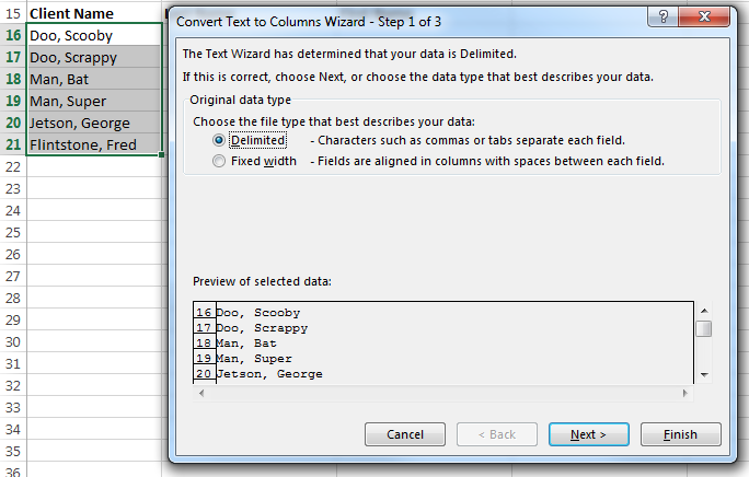
5. Place a check in the "Comma" Checkbox and deselect the others

6. Look at the Data Preview to see what the output will look like prior to proceding:

7. Click "Next"

8. This screen will allow you to format the text by column.  For this demonstration, we're happy with a               "General" format (the default).

9. In the Destination box, enter the location where you wish the first data point to appear.  In this case, let's select "$B$16" - just to the right of the names that we are using for this example. 

10. Click "Finish".

You should now see:

Enjoy!

UPPER CASE, lower case, Proper Case

Today's post is about changing the case of your source text to UPPER CASE, lower case, or Proper Case.

Formulas we'll need:
=Upper() - ALL CHARACTERS IN UPPER CASE
=Lower() - all characters in lower case
=Proper() - All Characters In Proper Case

Here we can see that we have a list of names.  Unfortunately, the names were simply entered without a specific format... Let's fix these:

In Cell B2 I'm entering "=Upper(A2)".
In Cell C2 I'm entering "=Lower(A2)".
In Cell D2 I'm entering "=Proper(A2)".

I then copy these formulas down to row 7 (or use auto-fill).  Here's what we have:

As you can see, the formulas convert the text just as they should.  So, how do we deal with this in a large table full of data?

1. Insert a new column (temporary) next to the column with the text you wish to convert
2. Use the desired formula in the uppermost cell (below the header) of the new column
3. Copy the formula down the column or use auto-fill
4. Copy the data in the new column
5. "Paste Special" > "Values Only" to the original column - this replaces the original data with the newly formatted data.
6. Delete the temporary column that you inserted,

Your data should now be formatted the way you want it.  As always, if there is a step that you are not familiar with, please let me know and I can further explain.