Favorite Excel Shortcut Keys

Hello all,

Here are a few of my most used/favorite short cut keys for Excel.  Not having to always rely on using the mouse has made me much more efficient in my work.

Quick Functions:

Ctrl + V = Paste
Ctrl + X = Cut
Ctrl + C = Copy

Ctrl + Z = Undo
Ctrl + Y = Redo
Ctrl + S = Save
Ctrl + O = Open
Ctrl + P = Print

Ctrl + B = Bold
Ctrl + I = Italicize
Ctrl + U = Underline

Ctrl + T = Open the Insert Table Dialog box
Ctrl + F = Find
Ctrl + H = Find/Replace

F2 - Open/Activate a cells contents for editing
Alt + F4 = Close Current Window

Tab - Close Cell Editing and move 1 cell to the Right
Enter - Close Cell Editing and move 1 cell Down

For movement without using the Mouse:

Arrow directional Keys (Up, Down, Left, Right) = Move 1 cell in that direction
Ctrl + Home = Goto Upper-Left most cell in spreadsheet
Ctrl + End = Goto Lower-Right most cell in spreadsheet
Ctrl + [Arrow direction Key] = Goto the end of column/row or next empty cell in that direction
Ctrl + PageUp = Spreadsheet Tab to the Left
Ctrl + PageDown = Spreadsheet Tab to the Right

For Highlighting Cells:

Use the Movement Keys above, but hold "Shift" as well.


For a comprehensive list of shortcuts, go to the following Microsoft Link:
http://office.microsoft.com/en-us/excel-help/excel-shortcut-and-function-keys-HP010073848.aspx

Numbers as text??

I was asked the other day about data exported from an access data base where the numbers where displayed as text values in Excel.  If you have ever run into this, you know that it's not a super simple task to change the format of those cells to "Number", because after you change the format type of the cells to "Number", you then have to activate the cell (F2) and exit the cell (Enter/Tab) for every cell.  So how do you get around this?

Let's use this example below:

Column A has Ages that are in a text format (notice the green triangle at the top-left of each cell - if you hover the cursor over this, excel will display a message that the numbers are in text format)

Simply add a new column next to the column you're working on (column B). In cell B2, type the formula "=A2*1".  Auto-fill or copy the formula down the column.

The result of the formula will provide you with the numeric format of the age.  Now you can simply copy the values in column B and "Paste Special > Values Only" in column A.  The age column values are now Numeric and no longer Text.

Delete the new column (Column B) to restore your data to it's original structure.

Dates and Pivot Tables

I was asked the other day how to show just the month within a pivot table row using a field that has dates formatted like "1/1/2014" throughout the year.  As I discussed this further, I found out that it would be useful to have the month show and then all of the dates within that month below it.

Today we're going to address methods to accomplish these tasks:

#1 - In a cell or cells, how do I show only the month in a year?  Let's Use "1/1/2014":

• =Text([cell reference with date value],"mmm") = Jan
• "m" = 1
• "mm" = 01
• "mmm" = Jan
• "mmmm" = January

• =Month([cell reference with date value])
• This will give the number of the month = 1]

• Right-click on column with the dates > Format cells > Number Tab > Custom > Type = "mmm" (use one of the above)

#2 - In a pivot table, how do I group the dates by month in the row category?

First, let's check to see that our data table is ready for a pivot table... What are we missing?  Well, in order for a pivot table to function properly and include all columns selected, each column must have a column header.  In this data set, we're missing the header in column A.  Let's add one and then insert our pivot table.

To insert a pivot table: Highlight your data table (A1:D9) > Insert > Pivot Table > New Worksheet > OK

Now, we're ready to include our dates in the Rows.  Add the "Date of Purchase" field to the Rows area:

The Resulting table looks like this:

Now, lets group by the date:

1. Click on a date in the pivot table
2. Right-click the same date you just selected
3. Click "Group..."
4. For this example, choose both "Months" and "Years" (**to de-select an item just click it again!) 
5. Click OK

**Tip: If you are getting an error when trying to click "Group...", check to make sure that none of your cells in your date column are blank.  Excel will not allow you to group with blank cells.

Now, Add the Price field to the values field in your pivot table.  Your pivot table will now look like this:

The above example shows us how to group the data by year and month.  

Now, how do we add the individual dates underneath the month?  For this, we will need to make some additions to our table.  Add the following formulas into the columns next to the table:

Auto-fill or copy/paste the formulas down to the end of the table.  

*I'm also going to change the bottom date value to 2/2/2014 for purposes of this example.

Use the following steps to create the desired table:

• Highlight the data table
• Insert Pivot Table on a New Worksheet
• Add (in this order) Year, Month, Date of Purchase to the rows section of the pivot table
• Add Price to the values section of the pivot table

You now have a pivot table that groups the data By Year, By Month AND has individual line items under the month.

Last, since we're looking at dollars, let's format the "Sum of Price" column as currency:

• Double-click on "Sum of Price" column header in the pivot table
• Click the "Number Format" button at the bottom of the Value Field Settings pop-up window
• Choose "Currency" and your preferred format for negative numbers
• Click "OK"

You now have this:

There are lots of great ways to make data more meaningful through the use of pivot tables.  In the future I will discuss using Power Pivot, data models, and slicers to be more efficient and effective in your work.

Creating a useful Process Chart (Using Excel 2013)

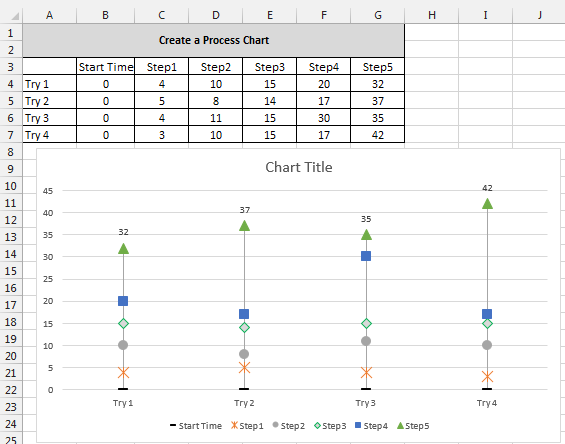
Today's post is about creating a Process Chart that will help you to visually identify areas of opportunity within a process.  I work within the healthcare industry.  It is often very important that we provide timely care in an effective manner.  The chart example below is something that I developed  for our team as we were trying to track times from patient arrival to the hospital to when each step was completed in our process, and ultimately, the time a given treatment was administered.  When you already have an idea of how long a process should take, it becomes a matter of comparing expected times with actual times and identifying where the delays occurred - these are the opportunities that need to be investigated further to see what was different/caused a variation in the process for that individual case.

Alright, enough chit-chat - Let's DO IT!

Example Data Set:
It is important to note, that when tracking times, the time for each step needs to be in relation to the "start time" or a common point of reference. In this case, start time = 0.

Create the Chart:
Highlight the Data Set (Cells A3:G7).
Click "Insert" Tab at the top
In "Charts", select the "Line With Markers" chart

Right-click the white chart area (Up near the title works)
Click "Select Data"
Click "Switch Row/Column" button - this will place the process steps in the "Series" column and the attempts in the "Category" column.

Look at the chart:

Add Lines to indicate time between steps:
Left-click the chart
Go up to "Chart Tools" > Design
Click "Add Chart Element" on the Ribbon > Lines > Drop Lines

Remove series lines but leave the markers:
Click a Series line (Step1, Step2, etc...) > Right-click on the series line
Click  "Format Data Series"

Click the paint can image and select "Line" in the options below the paint can.

Click the "No line" radio button

Look at the chart:

Repeat steps to remove line for remaining series (steps).

**Tip: If you do not close the "Format" pane after you select "No line", you can simply click on the next series line and format pane will remain open.  This will allow you to quickly go through each series and remove the lines without the "Right-click" steps.

Changing the Markers:
Click on a series marker on the chart - *Allow excel to select all of the markers in the series
Right-click on the marker
Click "Format Data Series"
Click the paint can image and select "Line" in the options below the paint can.
Below the paint can, click on "Marker"

Under "Marker Options" click the "Built-in" radio button

Change the "Type" to a square marker

**Tip: You may also adjust the size of the marker and in the "Fill" section below "Marker Options" you can change the marker fill as well as adjust the border in the "Border" section - Play around with it, see what you like!

Repeat above steps to make each series' marker unique (but the same across each series).

You chart should look similar to this:

Add Data Labels to the final step, or top data series, in the process to show total time:
Click the data series at the top of the chart (Mine is the green triangle)
Right-click the series
Click "Add Data Labels" > "Add Data Labels"
Click on a data label to select all of the labels
Right-click on the data label
Click "Format Data Labels..."
In the format pane on the right, select the bar graph icon
Under "Label Position" select the "Above" radio button.
The labels are now "above" the markers.

**Tip: You can format data labels by clicking on them and using the ribbon at the top "Home" > "Font"

Last, Lets jazz up the chart a bit and make it a bit more presentation ready:

Chart Title:
[Insert name of the process here]
Source: [name of data source]
Last Updated: [Date/Time data was last updated]

**All of this goes into the single title text box - Just add a carriage return to add a new line.  Once you've added the text, highlight the bottom two lines and change the font size to something like "8" to make it smaller.  It's important information, but we don't want it to distract from the chart itself.

Adding Axis Labels - Be sure to label your axes appropriately!
Click on chart
Go up to "Chart Tools" > Design
Click "Add Chart Element" on the Ribbon > Axis Titles > Primary Horizontal/Primary Vertical
Change the Vertical Axis' text to "Time (Minutes)" or something similar.

**I am not including a horizontal axis label since the data and legend are self explanatory

The Final Chart will look something like this:

As you can see, this can be a very useful chart that allows us to identify where opportunities exist within a time driven process.  It is very simple visually, and very easy to identify steps that are taking longer than others.  If you have used something similar or have another spin on this, please share in the comments below: how it was used and what industry you're working in.

VBA: Select Case

Alright VBA users... Have you ever needed to to use and if/then statement with multiple criteria and need to run a lot of code after the criteria is met?  Well, Select Case is the code for you!

It looks like this:

Select Case [What you are evaluating]
   Case is = [potential value]
       'your code goes here
   Case is = [potential value]
       'your code goes here
   Case is = [potential value]
       'your code goes here
   Case Else
       'your code goes here
End Select

Let's put it to use.  In this example, I am going to evaluate the value within cell B1.  In my code, I personally prefer using the "Cells()" reference method over the "Range()" reference method.  Cells(row, col) is what you'll see.

Select Case Sheets("Sheet1").cells(1, 2).value - This opens the "Select Case" Statement and shows that we're looking at the value of cell B1 or row1, column2.

Next, if the cell value is 1, 2, or 3 I want run specific code depending on the value.
Select Case Sheets("Sheet1").cells(1, 2).value
   Case is = 1
      [insert code here]
   Case is = 2
      [insert code here]
   Case is = 3   
      [insert code here]

So what if the cell value isn't 1-3?  Well, in that "case" (Pun!) you will use the "Case Else" Statement.

Select Case Sheets("Sheet1").cells(1, 2).value
   Case is = 1
      [insert code here]
   Case is = 2
      [insert code here]
   Case is = 3   
      [insert code here]
   Case Else
      [insert code here]

Finally, when you are done adding cases and code, you need to close the Select Case Statement with "End Select"

Select Case Sheets("Sheet1").cells(1, 2).value
   Case is = 1
      [insert code here]
   Case is = 2
      [insert code here]
   Case is = 3   
      [insert code here]
   Case Else
      [insert code here]
End Select

**Tips and tricks:
#1 - if you are going to be using VBA, pay attention to the formatting of the code.  Think of your code as an onion (multiple layers, not that they stink or make you cry).  Your opening statement is the outer layer (no indentation).  As you move into the statement - for example from the "Select Case ..." to "Case is =..." you will press tab and indent to indicate that what is happening is happening within the Select Case Statement. The code you include if a statement is True would be indented twice.  The "End Select" statement is referring to the "outer layer" so it is not indented to complete visual.

My code above in Blue is an example of this.

#2 - If you do not intend for anything to happen when a condition is met using the Select Case statement, simply do not place any code in the [insert code here] section and the program will resume by ending the select statement and continuing to the next line.

Locked out of my file!

Have you ever password protected an excel file (Sheet Protection, Workbook Protection) only to forget the password when someone needs you to make a change 2 years later?  Well, here's how to open it back up.

Open the file with Open Office Calc.  Yep, that's it! Simple as that. You will be able to un-protect what you need to and get on with your day.

Nice and easy, right?  On the flip side, it hopefully helps you realize just how vulnerable Excel data can be, so be careful.

Dollar Signs in formulas

Let's discuss using dollar signs in formulas.  What are they used for and how do we use them?

There are three different uses of dollars signs in formulas.  In cell B1 we will insert the different "$" formula references to cell A1:

1. =$A$1
2. =$A1
3. =A$1

What do these mean? 

1. =$A$1 - This means that if you copy this formula to any cell (example: D3) in any other column or row, it will still be and always be a reference to A1.
2. =$A1 - This means that the column reference will always be "A", but the row will change based on the row of the cell you're placing the formula in.  So, if you copy it to D3, then the value with show what is in $A3.
3. =A$1 - This means that the row reference will always be "1", but the column will change based on the row of the cell you're placing the formula in.  So, if you copy it to D3, then the value with show what is in D$1.

What do we use these for? Let's take a look:

In column "A" I have placed the values 1,2,3,4 in cells A1, A2, A3, A4.  The values in cells B1 to C4 will be the result of copying that formula to each of those cells.

=$A$1 

    No matter where the formula is copied (B1:C4), the result is the value in "A1"

=$A1

    The copied formula will always show a value from column "A", but the row will be based on the cell the formula is copied to.

For this next example, I changed the data a bit to show how the formula works.  The typed values are in cells A1, B1, C1, D1.  The formula will be copied to cells A2 to D5.

=A$1

    As you can see, the formula maintains the values in Row 1 (Row has the "$"), but changes with the columns (Column "A" does NOT have a "$").

In conclusion, the use of the dollar sign "$" is very useful when you are planning on having to copy the formula across multiple cells.  A properly placed "$" will allow you to ensure formula integrity.  

VBA Tip: Option Explicit

When I first started dabbling in writing my own macros I often saw the words "Option Explicit" before any code that was demonstrated on help sites.  I wondered what it was.

So what does "Option Explicit" mean?  Well, if you plan on using variables within your VBA code and inevitably you will, option explicit requires you to declare each variable.

How do I declare a variable?  The syntax for declaring a variable within VBA is:

Dim [your variable name] as [Type of variable]

An example:

Dim MyVar as Integer

So what do I get out of using Option Explicit you ask? When the code compiles prior to running, you will receive an error message if you have a variable that has not been declared.  This protects you from accidental typos of variables.

Using the example above, if I typed MVyar instead of MyVar and was not using Option Explicit -  as long as the typo is not one of the VBA reserved words, methods or properties - VBA would by default assign MVyar as a new variable.  This can make troubleshooting your code very difficult.

In conclusion, best practice states we should just set Option Explicit as a default setting.  Here's How (Using Excel 2013):

• Open an Excel Workbook > Open VBA (alt + F11)
• Tools > Options > "Editor" Tab
• Check "Require Variable Declaration"  (See picture below)

Question at work....

Okay folks, I found a winner yesterday while at work.  I was asked by a colleague if there was a way to sum the value of multiple items from an array off to the side of a data table. In other words, he wanted to find the values of items a,b,c within a data table that contains multiple occurrences of items a-z and their values.  It looks something like:

So, I Googled "Sum", "Criteria", "Array"

The formula that I eventually came up with was found @ http://www.mrexcel.com/forum/excel-questions/593233-sumif-criteria-array.html

The formula looks like: =SUM(SUMIF(A3:A11,{"a","b"},B3:B11))

The interesting thing about this formula, is that the criteria portion of the SumIf() formula is in {} and listed as an array.  However, it's important to note that so far as I've been able to find, you can't use cell references within that array - it will just give you an error and pop up a message. So, the values you're looking for, must be actually typed out and within quotes.

Something else I noticed as I was toying around with this formula was that if you leave off the outer "Sum() formula, the sumif() formula only returns the sum of the "a" values (=50).  When the Sum() is added around the SumIF() formula, all values within the criteria are added (=63).

Anyway, if anyone has further light to shed on this subject, please do so!  As I've said before we're all learning together.

Named Ranges: Dynamic Range for Chart Data Series

=OFFSET(Calcs!$I$1,1,0,(Counta(Calcs!$I$!:$I$1000)-COUNTIF(Calcs!$I$1:$I$1000,"")))

WHAT IS THIS?!?  Well, let's see...

I use this formula as the value for a named range on a spreadsheet that is nothing but formulas that are pulling data together from a "Raw Data" spreadsheet.

The formula essentially looks within the range I1:I1000 and defines the range that represents all cells with data in them, or are not equal to "" or blank.

Let's break it down by each formula used:

• =Offset(reference, rows, cols, [height], [width]) - Straight from the formula description: "Returns a reference to a range that is a specified number of rows and columns from a cell or range of cells. The reference returned can be a single cell or a range of cells." 
• =Counta(value1, value2...) - Used to count the number of cells within a range that contain text/formulas
• =Countif(range, criteria) - a conditional statement that allows you to count the number of cells that meet a single criteria that you've specified.

If we were to read the formula in simplified layman's terms we would say: Starting at cell I1 and staying within the same column, count the number of rows/cells that contain a value that is not blank or "".  Then return the overall range as the final calculated value.

This is why we can use this named range as a data series in a chart.  If the data grows, the formula recognizes that because another cell is no longer blank, and since the chart is using the named range with the formula, the data series reflects that.

One caveat to this formula, if you have a null value in the original data set, the cell value on the spreadsheet with the subset of data cannot = "" or blank.  It will need to read "Null" or "NA" or something of the like - otherwise the above formula stops when it finds the blank and will not reflect well in the chart.

Hope this helps!

VBA Tip for the day: Screen Updating

VBA - Screen Updating.

Have you ever created a macro that bounces between spreadsheets and causes the screen to flash because it's trying to keep up with the macro switching worksheets?  Well, there's a quick fix for that:

Option Explicit
Sub StopFlashing()
Application.ScreenUpdating = False

[Your code Here]

Application.ScreenUpdating = True
End Sub

This will not only stop the screen from flashing and causing your users to have seizures, but it will also help to optimize the macro and allow it to run faster!

Formula for the Day: =Sum(number1, number2 . . .)

"=sum( )"

The sum function in Excel is wonderful!

1. In the formula bar, type "=sum("
2. Select your range (what are you adding?) - Click on a cell or multiple cells, or a whole row/column
3. Close the formula with ")".
4. Press Enter

This will add all of the numerical data within the cell range(s) that you provided.  It's very simple and much faster than having to type =A1+A2+A3...

*You can also add items from multiple spreadsheets! after you select your first cell reference to add, simply type a comma "," to indicate that the next item is a new reference.  Select the spreadsheet tab at the bottom, select the cell with the number you're looking to add and presto! You've added two cells on two different spreadsheets.  - This method is especially handy if you're creating a summary page to provide a quick glance at high level data.

Hello World!

My name is Dan and I'm an Excel addict.  I absolutely love learning how to do new things in Microsoft Excel.  My specialties are in creating templates, dashboards, scorecards, automation of processes, analysis, and writing macros in VBA. Before I continue though, I'd like to share some of my favorite sources I've used over the years for my questions:

www.mrexcel.com
www.ozgrid.com
www.peltiertech.com

My goal for this blog is not to have a forum for users to ask for help, but to simply share some of the experiences and knowledge that I've gained over the years.  I will also add new formulas and how-to's for every level of user.  This is not a problem solving forum, so if you need help with a specific problem, try the sites listed above.

My journey toward Excel greatness began very simply... 10 years ago, I had a job I didn't like!  I was a unit clerk on a hospital unit and I wasn't very good at it and didn't really enjoy it.  For those that may be sympathizing at this point, there are a few choices available when you feel like you're backed into a corner and can't get out:

1. Curl up into a ball, cry, and blame everyone and everything around you.
2. Continue with the current situation
3. Get educated, make yourself better, and get the heck out of there!

Personally, I prefer #3 so I began by using the following process:
1. Finding a question
2. Asking the question
3. See it - Do it - Teach it.

1. Finding a Question:  Well, for my first "Big" Excel question, I wanted to know how to make the cells below my formula have a similar formula but for the cells in the row below (Sound familiar?)... In other words, I wanted to automatically fill ("AutoFill") the cells below my current, active cell with the same formula but have the references change with the row.  Yes, I wanted to use Auto-Fill.  No, I had never used it.

2. Asking the question: I've found the the biggest part of solving a problem is asking the right question. When I started on my quest for knowledge ten years ago, I knew enough to look in the help files - not really helpful, but enough to get me where I needed to go.  Nowadays, I prefer to consult "The Google" and see what results come back.  A tip for a good search is to determine what the key words are.  In the case of my first question, I would use the words Excel, Automatic, fill, and Formula [Give it a try and see what you get!]

3. See it, Do it, Teach it:  This is a method of learning that seems to work very well for me.  Everyone is different, but I find this is a pretty solid way to learn things.  See it: Watch how to do it, or read how to do it. Do it: Try it out! Teach it: Teaching someone else often requires a lot of forethought and detail oriented instruction.  If you can teach someone else to do it, you've got it figure out.

In closing, I'm hoping this blog will help others in their quest for knowledge.  I know that through hard work and dedication we can all become AWESOME in whatever we're trying to do.

Cheers!