Another quick post:
Have you ever had the wonderful pleasure of needing to pull all characters to the right of the 2nd or 3rd space within the string? I know I have..
Solution:
*Disclaimer*: I have no idea where I found this beauty, but again, I FOUND it because someone else was willing to share - and sharing is the whole point of this blog... I'm posting this just as much for myself as for anyone else. :)
Assuming your string is in cell C2:
=FIND(CHAR(1),SUBSTITUTE(C2," ",CHAR(1),LEN(C2)-LEN(SUBSTITUTE(C2," ",""))-n))
For n:
("n" determines the number of spaces)
0=1
1=2 etc...
Showing posts with label Formula. Show all posts
Showing posts with label Formula. Show all posts
Wednesday, March 18, 2015

Tuesday, April 15, 2014
INDEX() & MATCH() - the new VLOOKUP()!
Sorry it's been a while, but life and a full-time job have been crazy of late... Enough about me though, let's get to it!
The other day I was called into an issue where the user needed a formula that would look up the results of specific tests based on the month that they were run. He wanted to enter a month into a cell and the formulas would return the values of the tests for that month. In response, I created a demo spreadsheet (No Macros) to show him how to get the result he wanted.
His initial question was "Is there a way to do this VLOOKUP()?". Yes, this could be accomplished with VLOOKUP() assuming the tables were organized appropriately, but I wanted to introduce a new method. VLOOKUP()is a great formula, but has it's limitations. For example, Column1 of the table referenced when looking for a specific value MUST be the left-most array column that contains that value...
While I'm sure there would be a convoluted way to go about accomplishing that task by counting the month from an original start date and using that as the column reference in the VLOOKUP() formula, I felt it would be a better time to use the INDEX() and MATCH() formulas to find the intersections of row and column.
Here's how I accomplished it:
Formulas:
INDEX(array, row_num, [column_num])
MATCH(lookup_value, lookup_array, [match type])
Data Set:
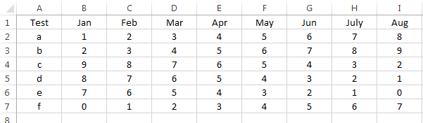
The user's file was set up so the column contains the test name (run only once per month and not duplicated) and the following columns are the results of the tests under each month.
Now, off to the right of the data set, I created an example of how to set up a quick reference for the month's data:
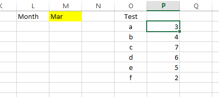
The Yellow cell is where the month is entered and cells P2:P7 contain the formulas that refer to the month and test name to return the appropriate value.
On to the formula... In cell P2, Start with the INDEX() formula. The array is the data table in cells A1:I7 so we now have:
=INDEX($A$2:$I$7,
The next step is to identify which row we're interested in. We use the MATCH() formula for this. The items we need for MATCH() are:
Lookup_value = O2 (this is the name of the test in question found in column "O")
Lookup_array = A2:A7 (This is the column containing the test names)
Match_type = 0 (zero - this means "Exact match with lookup_value)
So now we have:
=INDEX($A$2:$I$7,MATCH(O2,$A$2:$A$7,0)
Next, we need the column reference. Again, we use the MATCH() formula for this. The items we need for MATCH() are:
Lookup_value = M1 (this is the name of the test in question found in column "O")
Lookup_array = A1:I1 (This is the row containing the month names)
Match_type = 0 (zero - this means "Exact match with lookup_value)
Now, we have a completed formula in cell P2. Prior to copying the formula down, be sure to add the "$" where you need it to keep the references from shifting when they shouldn't - See the "Dollar Signs in Formulas" post if this doesn't make sense.
Final Formula:
=INDEX($A$2:$I$7,MATCH(O2,$A$2:$A$7,0),MATCH($M$1,$A$1:$I$1,0))
Now, when you change the Month in the yellow cell, the formula will match that month with each of the results and return the intersection or result of the test!
Now, I understand that this is not the only way to accomplish this task, nor is it the only way to use these formulas, but it IS the way I chose to solve the user's issue.
The other day I was called into an issue where the user needed a formula that would look up the results of specific tests based on the month that they were run. He wanted to enter a month into a cell and the formulas would return the values of the tests for that month. In response, I created a demo spreadsheet (No Macros) to show him how to get the result he wanted.
His initial question was "Is there a way to do this VLOOKUP()?". Yes, this could be accomplished with VLOOKUP() assuming the tables were organized appropriately, but I wanted to introduce a new method. VLOOKUP()is a great formula, but has it's limitations. For example, Column1 of the table referenced when looking for a specific value MUST be the left-most array column that contains that value...
While I'm sure there would be a convoluted way to go about accomplishing that task by counting the month from an original start date and using that as the column reference in the VLOOKUP() formula, I felt it would be a better time to use the INDEX() and MATCH() formulas to find the intersections of row and column.
Here's how I accomplished it:
Formulas:
INDEX(array, row_num, [column_num])
MATCH(lookup_value, lookup_array, [match type])
Data Set:
The user's file was set up so the column contains the test name (run only once per month and not duplicated) and the following columns are the results of the tests under each month.
Now, off to the right of the data set, I created an example of how to set up a quick reference for the month's data:
The Yellow cell is where the month is entered and cells P2:P7 contain the formulas that refer to the month and test name to return the appropriate value.
On to the formula... In cell P2, Start with the INDEX() formula. The array is the data table in cells A1:I7 so we now have:
=INDEX($A$2:$I$7,
The next step is to identify which row we're interested in. We use the MATCH() formula for this. The items we need for MATCH() are:
Lookup_value = O2 (this is the name of the test in question found in column "O")
Lookup_array = A2:A7 (This is the column containing the test names)
Match_type = 0 (zero - this means "Exact match with lookup_value)
So now we have:
=INDEX($A$2:$I$7,MATCH(O2,$A$2:$A$7,0)
Next, we need the column reference. Again, we use the MATCH() formula for this. The items we need for MATCH() are:
Lookup_value = M1 (this is the name of the test in question found in column "O")
Lookup_array = A1:I1 (This is the row containing the month names)
Match_type = 0 (zero - this means "Exact match with lookup_value)
Now, we have a completed formula in cell P2. Prior to copying the formula down, be sure to add the "$" where you need it to keep the references from shifting when they shouldn't - See the "Dollar Signs in Formulas" post if this doesn't make sense.
Final Formula:
=INDEX($A$2:$I$7,MATCH(O2,$A$2:$A$7,0),MATCH($M$1,$A$1:$I$1,0))
Now, when you change the Month in the yellow cell, the formula will match that month with each of the results and return the intersection or result of the test!
Now, I understand that this is not the only way to accomplish this task, nor is it the only way to use these formulas, but it IS the way I chose to solve the user's issue.
Tuesday, March 25, 2014
Guest Contribution: Formula to Show Beginning of Week
Hey all! Today's post is provided by guest contributor Jerry Shelton. Jerry is a Project Manager at Hewlett Packard as well as an HP Sigma Plus Certified Black Belt. Lucky for us, he has provided a wonderful example of how to take a date/time stamp from a data set that was exported from a database and determine the beginning of the week to allow for simple grouping within a pivot table/chart.
This solution is a real-world example that was born out of the need of others that were not too excel savvy to create reports from data sources with similar formatting. This template allows them to simply copy/paste the formulas shown in this example into their own data and move from there with very little training or guidance from others. I fully support making life easier for others!
Here's a link to the file with the "How To" included inside:
Beginning of Week - Formula Example
**Note: The above file does not contain Macros.
Cheers!
This solution is a real-world example that was born out of the need of others that were not too excel savvy to create reports from data sources with similar formatting. This template allows them to simply copy/paste the formulas shown in this example into their own data and move from there with very little training or guidance from others. I fully support making life easier for others!
Here's a link to the file with the "How To" included inside:
Beginning of Week - Formula Example
**Note: The above file does not contain Macros.
Cheers!
Wednesday, February 12, 2014
UPPER CASE, lower case, Proper Case
Today's post is about changing the case of your source text to UPPER CASE, lower case, or Proper Case.
Formulas we'll need:
=Upper() - ALL CHARACTERS IN UPPER CASE
=Lower() - all characters in lower case
=Proper() - All Characters In Proper Case
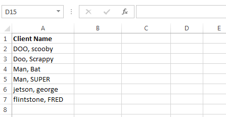
Here we can see that we have a list of names. Unfortunately, the names were simply entered without a specific format... Let's fix these:
In Cell B2 I'm entering "=Upper(A2)".
In Cell C2 I'm entering "=Lower(A2)".
In Cell D2 I'm entering "=Proper(A2)".
I then copy these formulas down to row 7 (or use auto-fill). Here's what we have:
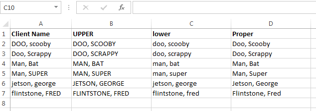
As you can see, the formulas convert the text just as they should. So, how do we deal with this in a large table full of data?
Formulas we'll need:
=Upper() - ALL CHARACTERS IN UPPER CASE
=Lower() - all characters in lower case
=Proper() - All Characters In Proper Case
Here we can see that we have a list of names. Unfortunately, the names were simply entered without a specific format... Let's fix these:
In Cell B2 I'm entering "=Upper(A2)".
In Cell C2 I'm entering "=Lower(A2)".
In Cell D2 I'm entering "=Proper(A2)".
I then copy these formulas down to row 7 (or use auto-fill). Here's what we have:
As you can see, the formulas convert the text just as they should. So, how do we deal with this in a large table full of data?
- Insert a new column (temporary) next to the column with the text you wish to convert
- Use the desired formula in the uppermost cell (below the header) of the new column
- Copy the formula down the column or use auto-fill
- Copy the data in the new column
- "Paste Special" > "Values Only" to the original column - this replaces the original data with the newly formatted data.
- Delete the temporary column that you inserted,
Your data should now be formatted the way you want it. As always, if there is a step that you are not familiar with, please let me know and I can further explain.
Friday, December 27, 2013
Dollar Signs in formulas
Let's discuss using dollar signs in formulas. What are they used for and how do we use them?
There are three different uses of dollars signs in formulas. In cell B1 we will insert the different "$" formula references to cell A1:


There are three different uses of dollars signs in formulas. In cell B1 we will insert the different "$" formula references to cell A1:
- =$A$1
- =$A1
- =A$1
What do these mean?
- =$A$1 - This means that if you copy this formula to any cell (example: D3) in any other column or row, it will still be and always be a reference to A1.
- =$A1 - This means that the column reference will always be "A", but the row will change based on the row of the cell you're placing the formula in. So, if you copy it to D3, then the value with show what is in $A3.
- =A$1 - This means that the row reference will always be "1", but the column will change based on the row of the cell you're placing the formula in. So, if you copy it to D3, then the value with show what is in D$1.
What do we use these for? Let's take a look:
In column "A" I have placed the values 1,2,3,4 in cells A1, A2, A3, A4. The values in cells B1 to C4 will be the result of copying that formula to each of those cells.
=$A$1
No matter where the formula is copied (B1:C4), the result is the value in "A1"
=$A1
The copied formula will always show a value from column "A", but the row will be based on the cell the formula is copied to.
For this next example, I changed the data a bit to show how the formula works. The typed values are in cells A1, B1, C1, D1. The formula will be copied to cells A2 to D5.
=A$1
As you can see, the formula maintains the values in Row 1 (Row has the "$"), but changes with the columns (Column "A" does NOT have a "$").
In conclusion, the use of the dollar sign "$" is very useful when you are planning on having to copy the formula across multiple cells. A properly placed "$" will allow you to ensure formula integrity.
Saturday, December 21, 2013
Question at work....
Okay folks, I found a winner yesterday while at work. I was asked by a colleague if there was a way to sum the value of multiple items from an array off to the side of a data table. In other words, he wanted to find the values of items a,b,c within a data table that contains multiple occurrences of items a-z and their values. It looks something like:

So, I Googled "Sum", "Criteria", "Array"
The formula that I eventually came up with was found @ http://www.mrexcel.com/forum/excel-questions/593233-sumif-criteria-array.html
The formula looks like: =SUM(SUMIF(A3:A11,{"a","b"},B3:B11))
The interesting thing about this formula, is that the criteria portion of the SumIf() formula is in {} and listed as an array. However, it's important to note that so far as I've been able to find, you can't use cell references within that array - it will just give you an error and pop up a message. So, the values you're looking for, must be actually typed out and within quotes.
Something else I noticed as I was toying around with this formula was that if you leave off the outer "Sum() formula, the sumif() formula only returns the sum of the "a" values (=50). When the Sum() is added around the SumIF() formula, all values within the criteria are added (=63).
Anyway, if anyone has further light to shed on this subject, please do so! As I've said before we're all learning together.

So, I Googled "Sum", "Criteria", "Array"
The formula that I eventually came up with was found @ http://www.mrexcel.com/forum/excel-questions/593233-sumif-criteria-array.html
The formula looks like: =SUM(SUMIF(A3:A11,{"a","b"},B3:B11))
The interesting thing about this formula, is that the criteria portion of the SumIf() formula is in {} and listed as an array. However, it's important to note that so far as I've been able to find, you can't use cell references within that array - it will just give you an error and pop up a message. So, the values you're looking for, must be actually typed out and within quotes.
Something else I noticed as I was toying around with this formula was that if you leave off the outer "Sum() formula, the sumif() formula only returns the sum of the "a" values (=50). When the Sum() is added around the SumIF() formula, all values within the criteria are added (=63).
Anyway, if anyone has further light to shed on this subject, please do so! As I've said before we're all learning together.
Wednesday, December 18, 2013
Formula for the Day: =Sum(number1, number2 . . .)
"=sum( )"
The sum function in Excel is wonderful!
- In the formula bar, type "=sum("
- Select your range (what are you adding?) - Click on a cell or multiple cells, or a whole row/column
- Close the formula with ")".
- Press Enter
This will add all of the numerical data within the cell range(s) that you provided. It's very simple and much faster than having to type =A1+A2+A3...
*You can also add items from multiple spreadsheets! after you select your first cell reference to add, simply type a comma "," to indicate that the next item is a new reference. Select the spreadsheet tab at the bottom, select the cell with the number you're looking to add and presto! You've added two cells on two different spreadsheets. - This method is especially handy if you're creating a summary page to provide a quick glance at high level data.
Subscribe to:
Posts (Atom)