Rolling 12 Months Chart

I know I haven't posted in a while... I've been crazy busy with work, moving, and life in general.. But things are settling down and I hope to get back on track.

Recently I was asked to create a chart that could function as a "rolling 12 months" chart.  If using Power Pivot in Excel 2010 or 2013, this would have been quick and easy using a date/time dimension table to slice the data.  However, this needed to be supported in Excel 2007.  Soooo, I had to get creative.

Here is what I came up with -

Specific formulas needed:
=EDATE(start date, months)
=VLOOKUP(Lookup value, table array, col_index_num, [range_lookup])

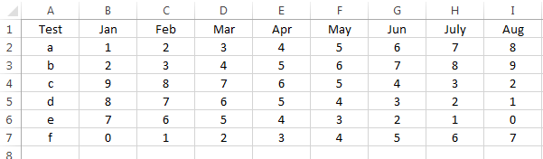
To begin, we have our data set:

This is simply a random data set that I generated for this example with no true significance in the real world... Note: The dates in column "A" were entered as "6/1/2012" and then formatted within the cell to only show month/year.  I always use the first day of the month when working with month-year formats.  Not sure if this is best practice, but it is my own standard since there is always a day "1" in every month.

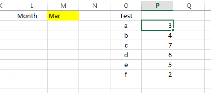
Next, I created a table that will show the 12 months' data:

Above the table I simply added "Last Month" and "Last Year" fields for data entry.  These will be used by formulas within the table.  The numbers in the yellow cells are manually entered/changed - although I suppose you could use a data validation drop-down if you wanted to limit what could be entered.

Anyway, Here's how I created the table:
In the bottom left cell of the table ("Jun-14") I added the formula: =DATE(I1, G1, 1) where G1 is the value entered in the yellow cells for "Last Month" and I1 is the value entered in the other yellow cell for "Last Year" - Last month and Last year meaning the last month/year you wish to be shown on the chart.

In the cell above the "Jun-14" cell, I use the formula: =EDATE(F14,-1) where F14 is the date that we just created in the bottom left cell of the table, and "-1" tells excel to subtract 1 month.

I simply continue or "Auto-Fill" the formula to the top of the table.  Now, when you change the date parts in the yellow cells, the dates in the table will automatically adjust.

Next, we use a vlookup formula to go and gather the data that corresponds with the date in the first column of the table. By using the "dynamic" dates we've created, our data will also be dynamically selected from the original data set. - Since I've addressed vlookup in past posts, I'll skip this part.  I will post a snapshot of the table showing the formulas at the end though.

The last column in the table is simply a preference.  I create the numerator/denominator for the data label on the chart.  I do this simply by concatenating the values using this formula: =H3&"/"&I3 (this results in the value at the top right of the table: 1091/1100).  I find it very helpful to include the n/d when displaying percentages in a chart.  This shows the reader if 50% is 1/2 or 500/1000.

Final Snapshot of table showing formulas:

Last, I create a simple line chart using the "Month" and "Success%" columns in our table.  Add data labels to each of the data points on the chart.  To create dynamic chart data point labels simply click on an individual label, and in the formula bar type "=" and the cell reference of the value you are looking to display - In this case, the first label on the left would be =$J$3.

Since we created the table using relative references instead of specific numbers and values, when the Last Month and Last Year are changed at the top, the data in the table as well as the data on the chart are instantly updated to show the "rolling 12 months".

I know this was a bit rushed...  That's why I'm including an example file this time!  You can get it here.

INDEX() & MATCH() - the new VLOOKUP()!

Sorry it's been a while, but life and a full-time job have been crazy of late... Enough about me though, let's get to it!

The other day I was called into an issue where the user needed a formula that would look up the results of specific tests based on the month that they were run.  He wanted to enter a month into a cell and the formulas would return the values of the tests for that month.  In response, I created a demo spreadsheet (No Macros) to show him how to get the result he wanted.

His initial question was "Is there a way to do this VLOOKUP()?".  Yes, this could be accomplished with VLOOKUP() assuming the tables were organized appropriately, but I wanted to introduce a new method. VLOOKUP()is a great formula, but has it's limitations.  For example, Column1 of the table referenced when looking for a specific value MUST be the left-most array column that contains that value...

While I'm sure there would be a convoluted way to go about accomplishing that task by counting the month from an original start date and using that as the column reference in the VLOOKUP() formula, I felt it would be a better time to use the INDEX() and MATCH() formulas to find the intersections of row and column.

Here's how I accomplished it:

Formulas:
INDEX(array, row_num, [column_num])
MATCH(lookup_value, lookup_array, [match type])

Data Set:

The user's file was set up so the column contains the test name (run only once per month and not duplicated) and the following columns are the results of the tests under each month.

Now, off to the right of the data set, I created an example of how to set up a quick reference for the month's data:

The Yellow cell is where the month is entered and cells P2:P7 contain the formulas that refer to the month and test name to return the appropriate value.

On to the formula... In cell P2, Start with the INDEX() formula.  The array is the data table in cells A1:I7 so we now have:

=INDEX($A$2:$I$7,

The next step is to identify which row we're interested in.  We use the MATCH() formula for this.  The items we need for MATCH() are:

Lookup_value = O2 (this is the name of the test in question found in column "O")
Lookup_array = A2:A7 (This is the column containing the test names)
Match_type = 0 (zero - this means "Exact match with lookup_value)

So now we have:

=INDEX($A$2:$I$7,MATCH(O2,$A$2:$A$7,0)

Next, we need the column reference. Again, we use the MATCH() formula for this. The items we need for MATCH() are:

Lookup_value = M1 (this is the name of the test in question found in column "O")
Lookup_array = A1:I1 (This is the row containing the month names)
Match_type = 0 (zero - this means "Exact match with lookup_value)

Now, we have a completed formula in cell P2.  Prior to copying the formula down, be sure to add the "$" where you need it to keep the references from shifting when they shouldn't - See the "Dollar Signs in Formulas" post if this doesn't make sense.

Final Formula:

=INDEX($A$2:$I$7,MATCH(O2,$A$2:$A$7,0),MATCH($M$1,$A$1:$I$1,0))

Now, when you change the Month in the yellow cell, the formula will match that month with each of the results and return the intersection or result of the test!


Now, I understand that this is not the only way to accomplish this task, nor is it the only way to use these formulas, but it IS the way I chose to solve the user's issue.